Examples

This module contains example(s) of solving boundary value problems using the bvp package.

scikits.bvp1lg.examples.bessel_colnew()

Examples

Let’s use colnew to solve a multi-point boundary value problem for the Bessel differential equation and another coupled differential equation:

u''(x) = -u'(x) / x + (nu**2/x**2 - 1) * u(x)        for 1 <= x <= 10
u(1)  = J_{nu}(1)
u(10) = J_{nu}(10)

v'(x) = x**(nu+1) * u(x)                             for 1 <= x <= 10
v(5)  = 5**(nu+1) * J_{nu+1}(5)

First import numpy and bvp

>>> import numpy as np
>>> import scipy.special as special

>>> import scikits.bvp1lg.colnew as colnew

Then specify the equation system

>>> nu = 3.4123

>>> degrees = [2, 1]
>>> def fsub(x, z):
...     u, du, v = z     # it's neat to name the variables
...     return np.array([-du/x + (nu**2/x**2 - 1)*u, x**(nu+1) * u])

Here, fsub is vectorized over x: x has shape (nx,) and z shape (mstar, nx), where mstar = 3 is the number of free variables: u, du and v. fsub should return a vector of shape (ncomp, nx) where ncomp is the number of equations.

The partial derivatives wrt. variables can be provided, to gain speed

>>> def dfsub(x, z):
...     u, du, v = z
...     zero = np.zeros(x.shape)
...     return np.array([[(nu**2/x**2 - 1), -1/x, zero],
...                     [       x**(nu+1), zero, zero]])

zero is needed due to vectorizing.

The boundary points must be sorted:

>>> boundary_points = [1, 5, 10]

and the boundary conditions given in form

>>> def gsub(z):
...     u, du, v = z
...     return np.array([u[0] - special.jv(nu,   1),
...                     v[1] - 5**(nu+1) * special.jv(nu+1, 5),
...                     u[2] - special.jv(nu,   10)])

Here, z[i,j] is the value of variable i at boundary point j. Note that only separated boundary conditions are supported: condition at point j may only refer to z[:,j].

Again, the partial derivatives can be provided

>>> def dgsub(z):
...     return np.array([[1, 0, 0],
...                     [0, 0, 1],
...                     [1, 0, 0]])

dgsub(z)[i,:] contains the partial derivative of the boundary condition at boundary point i versus the three variables.

Then solve the problem (it is linear)

>>> tol = [1e-5, 0, 1e-5]
>>> solution = colnew.solve(
...     boundary_points, degrees, fsub, gsub,
...     dfsub=dfsub, dgsub=dgsub,
...     is_linear=True, tolerances=tol,
...     vectorized=True, maximum_mesh_size=300)

To satisfy the tolerances, we needed to increase the maximum mesh size from the default 100 to 300. The actual final mesh has 117 points:

>>> solution.nmesh
117

Finally, check that the u variable indeed is J_nu(x)

>>> x = np.linspace(1, 10, 101)
>>> np.allclose(solution(x)[:,0], special.jv(nu, x),
...            rtol=1e-4, atol=1e-8)
True

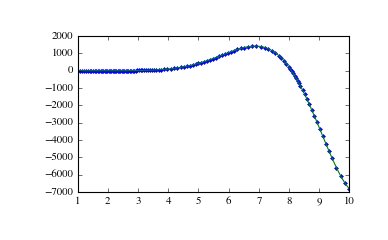
Due to a property of the Bessel functions, v(x) = x**(nu+1) J_{nu+1}(x)

>>> np.allclose(solution(x)[:,2], x**(nu+1)*special.jv(nu+1, x),
...            rtol=1e-4, atol=1e-8)
True

Note that in this case the algorithm slightly underestimated the errors: the solutions do not satisfy the specified tolerance 1e-5, although they satisfy the tolerance 1e-4.

Finally, we can plot the result:

>>> import matplotlib.pyplot as plt
>>> plt.plot(solution.mesh, solution(solution.mesh)[:,2], '.',
...          x, x**(nu+1)*special.jv(nu+1, x), '-')
[...]
>>> plt.show()